VHDL Design Creation/Verification mit Libero

This documentation was created as part of my seminar presentation in the winter semester of 2004/2005 (FH Wedel).

3. ActGen Core Builder - Working with Macros
1. Introduction
2. Structure of the program interface
3. Example: How do I integrate a counter into my HDL design?
4. Schematic Based Entry
1. Introduction
2. The interface of ViewDraw AE
3. An example design - working with ViewDraw
• Step 1: Create a new schematic file
• Step 2: Add components
• Step 3: Copy components
• Step 4: Connect components
• Step 5: Define inputs and outputs (I/O)
• Step 6: Add comments and graphic elements
• Step 7: Generate and integrate a counter (ACTgen Core)
• Step 8: Manipulate objects
• Step 9: Create a bus
• Step 10: Save and test the circuit
4. Special functions in ViewDraw AE
• Using multiple schematic worksheets (multi-page)
• What are Fubes?
• Create and integrate new symbols
5. Stimulus / Testbench - WaveFormer Lite
1. Introduction
• Starting the program from Libero
• Defining startup options
2. The graphical interface of WaveFormer Lite
3. Important options
• Setting the base time unit
• Display time unit
4. Working with WaveFormer Lite
• Adding and removing signals
• Defining signal properties
• Defining a clock signal
• Adjusting clock settings
• Copying and moving signals
• Drawing signal waveforms
• Adding a bus
• Time button and delta button
5. Import/Export - testbench generation
6. Outlook on the PRO version
7. Functional simulation
• Starting ModelSim from Libero
• Simulation options
6. Synthesis
1. Introduction
2. The interface of Synplify
3. The synthesis process
7. Notes on the tools
1. Fixing errors in an exported testbench
2. Source of error: testbench export format
3. Source of error: ModelSim does not display output signals
4. Source of error: ViewDraw does not start from within Libero
8. Help and further information
1. Useful documents on "Libero Design Creation/Verification"
2. Links to the tool manufacturers
3. Useful links related to VHDL

 

Introduction and Overview

What is "Design Creation / Verification" about?

When a new hardware project is carried out, the process begins after the preparation phase with the behavioral description of the desired functions:

Design Creation:
In Actel Libero, this can be done either by writing HDL code (VHDL or Verilog) (-> Text Based Entry). Another option is the supplied tool View Draw AE, which allows the functionality to be represented through a graphical interface by "clicking together" the design. (-> Schematic Based Entry).

Once the design or a sub-function has been fully described, the correct functionality of the unit must be verified. This is done with the help of testbenches that generate specific signal states so that the result can be verified.

Design Verification:
In Actel Libero, independently written VHDL testbenches can be used for simulation. With the help of the included and somewhat limited "Lite version" of SynaptiCAD WaveFormer, specific test sequences can be entered graphically via a waveform interface and then exported as a VHDL testbench. This can significantly simplify and shorten the testing and debugging phase. Once a testbench for the desired function is available, the behavioral simulation of the design can be started in ModelSim AE.

 

Associated design flow in Libero

The design flow in the area of design creation/verification consists of the following phases:

1. HDL design entry

• Entering the design in a text editor (HDL editor) or by using the graphical interface in View Draw AE (schematics).
• Creating and integrating (instantiating) ACTgen macros

2. Functional simulation

• Creating a standard HDL testbench with typical non-synthesizable elements (non RTL) such as "wait for" or "sig <= value after time", or generating one via waveforms with the additional program "WaveFormer Lite"
• Performing a functional simulation before synthesis to verify the functionality of the HDL code -> stimulus simulation with the additional program "ModelSim"
• Evaluation of the simulation results: debugging, improvements...

3. Synthesis / EDIF generation

• After the design has been created and correct functionality has been verified, synthesis follows by calling an additional program.
• The synthesis tool transforms the behavioral description (behavioral HDL) into a gate-level netlist and optimizes the design for the target platform.
• Pure schematic designs are automatically converted into a netlist by the Libero tool

The following figure illustrates the design flow in Libero once again:

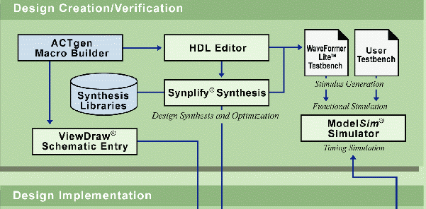
The Libero IDE supports the design flow and enables quick access to the various tools. The table below shows which tools are used during the "Design Creation/Verification" phase:

Function	Tool	Company
Project Manager, HDL Editor	Libero IDE	Actel
Schematic Capture	ViewDraw AE	Mentor Graphics
Synthesis	Synplify AE	Synplicity
Simulation	ModelSim AE	Mentor Graphics
Testbench Creation	WaveFormer Lite AE	SynaptiCAD
Physical Synthesis	PALACE AE	Magma Design Automation

Creating a new project

After starting the Actel Libero software, the workspace is initially empty. The menu item "File->New Project" opens the "New Project Wizard", which is used to configure and create a new project step by step:

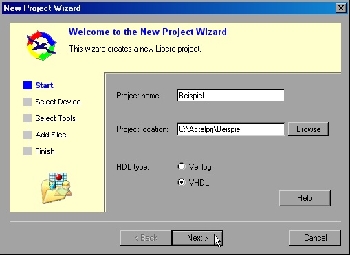
During the individual steps, the project name and type, storage location, target device, third-party tools to be used, and optionally existing files must be specified.
A click on "Finish" creates the project - design entry can begin!

The interface (IDE) in Libero

The Libero interface consists of three window areas embedded in the main program. An additional toolbar provides quick access to important basic functions such as loading and saving files without having to go through the menu:

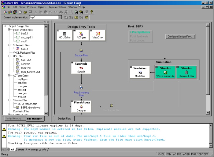
On the left side there is the "Design Hierarchy" together with the "File Manager", which displays all project files in a tree structure. A tab allows switching between the two views. On the right side the design flow is displayed, providing buttons for all relevant functions such as creating a new HDL file or launching the simulator. This is also the area for editing HDL files. Here too, switching is possible via the lower tab. The lower window is reserved for log and status messages, which can all be displayed or filtered (only errors, only warnings, or only info).

In addition, various actions are made possible by launching third-party programs, such as schematic design. For this purpose, the respective program is started from the IDE.

back to table of contents

---

Text Based Entry

Introduction

A suitable text editor is required for entering new designs textually or editing existing designs. The Libero interface includes a built-in editor that supports the hardware description languages VHDL and Verilog and can display code in both languages with syntax highlighting. Alternatively, any external editor (such as SciTE, UltraEdit or Notepad) can be specified. Once a new project has been created, you can begin creating and writing your own designs. However, it is advisable to define the most important settings first.

Editor selection and options

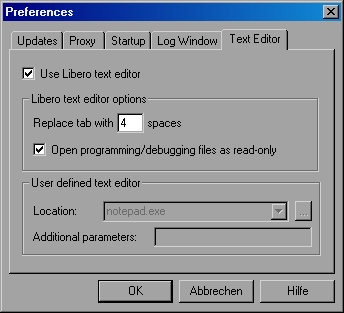
The settings dialog is displayed via the menu item "Files->Preferences...". After clicking the "Text Editor" selection field, either the editor integrated in Libero can be activated "->Use Libero Text Editor", or an external editor can be defined "->User defined text editor" (to do so, the check mark in the "Use Libero text editor" checkbox must be removed).

Creating, opening and importing HDL files

Create new HDL files

After the project has been created and the most important options have been set, a new HDL file can be created. The following steps are required:

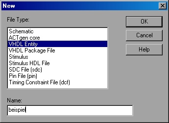
1. Select the menu item "File->New" (or the corresponding button in the design flow)
2. Click on "VHDL Entity", enter the file name in the lower "Name" field, and confirm with "OK" (the file extension can be omitted; it will be added automatically). The HDL editor opens, the design can be edited and saved via the menu item "File->Save". The new file has been added to the project and appears in the Libero "File Manager".

Open or import HDL files

Open files:
A HDL source file can be opened via the menu item "File->Open..." and then edited in the editor. In the open dialog, the file type "HDL File (*.vhd, *.vhdl)" should be selected. Files opened this way are not added to the current project; they are only edited.

Import files:
If a file is to be included in the project, this can be done via the menu item "File->Import Files...". A copy of the selected file is created in the project directory and included in the project hierarchy.

Special features of the integrated HDL editor

Multiple open files:
The Libero HDL editor supports multiple open files, each of which can be selected for editing via a tab.

Standard editing functions:
Standard Windows editing functions such as copy/paste etc. are available via keyboard shortcuts or the right-click context menu.

Commenting / uncommenting:
If one or more lines in the HDL code need to be commented or uncommented, this is most easily done with the comment function ("Comment out" or "Uncomment out"), which can be accessed either via the Edit menu or the right-click context menu.

Syntax checker

After writing an HDL file, it is useful to check the HDL code for correct syntax. Actel Libero provides the following function for this:

1. Important: All changes to the open HDL file must be saved (Ctrl+S).
2. In the Libero "File Manager", right-click the file to be checked and select "Check HDL File".

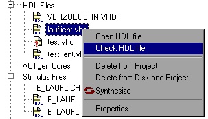
The file is checked and any existing syntax errors are displayed in the lower log window.

back to table of contents

---

ActGen Core Builder - Working with Macros

Introduction

With the ACTgen Core Builder, Actel Libero offers the possibility to integrate many frequently used functions such as counters, shift registers, adders or multiplexers into your own design. The desired function can be selected in a graphical interface, parameterized, and generated either as a netlist (EDIF, VHDL, Verilog) or as a behavioral model (for simulation purposes). The generated macros (cores) can be integrated both as symbols in schematic designs and in purely text-based designs.

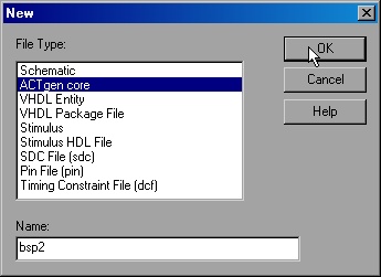
A new macro can be created via the menu item "File->New" or more easily with the "ACTgen Button" in the design flow. After entering a name and clicking "OK", the Core Builder is started as a new program. There, the macros are created with the desired options and automatically added to the project.

Structure of the program interface

As the following screenshot demonstrates, the interface is divided into four areas:

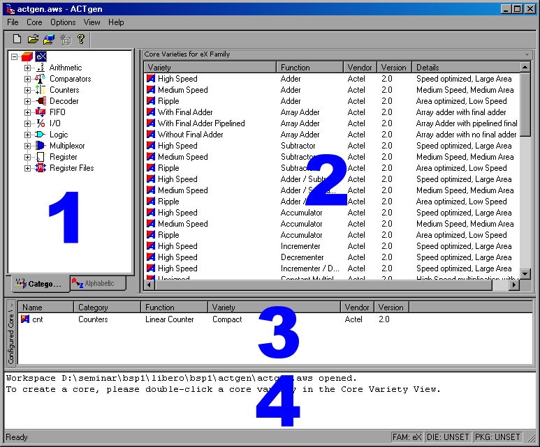
(1) Core Catalog:
This window displays all macros (cores) available for the currently selected hardware target platform (either grouped by category or sorted alphabetically). The desired element can be selected in the tree view.

(2) Variety View window:
If an element in the catalog is selected, this window lists the possible variations matching the selection (for example, if "Counters" is selected in the catalog, options such as "Sklansky, Fast Brent-Kung, Ripple..." are available here). Double-clicking the desired element opens a dialog for parameterizing and generating the core.

(3) Configured Core View window:
This window (workspace) displays all already configured cores and allows them to be modified or removed via right-click.

(4) Log window:
The log window displays information about the configured cores.

Example: How do I integrate a counter into my HDL design

The following example demonstrates the generation and integration of ACTgen cores into a VHDL design for the device "eX256-128CS". The goal is to design a counter that counts from 0 to 7 (3 bits), then automatically resets and starts again from the beginning. The counter is not described by the programmer in VHDL code, but is instead generated using a macro, adapted to the required needs, and finally integrated into the project in VHDL.

Step 1:
Create the VHDL file in which the macro is to be used (this will not be discussed in more detail here, as the previous chapter describes how a VHDL design can be created).

Step 2:
Create a new core for the counter: In the main Libero window, click the ACTgen button in the design flow (shown on the left). In the dialog that opens, select "ACTgen Core" and enter a name (for example "my_cnt"). After confirming, the ACTgen Core Builder is loaded and appears on the screen.

Step 3:
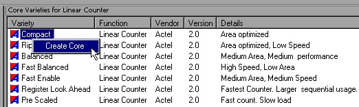
As shown in the screenshot, the desired function must now be selected in the left "Core Catalog" window. For our counter, we choose "Counters->Linear Counter". The supported variations are then listed in the right window. The "Details" column explains the differences:

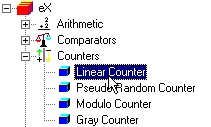
Step 4:
Once one of the offered variations has been selected (for this example, "Compact" was chosen), it is highlighted. Then, using the right-click context menu, "Create Core" can be selected, which opens a new dialog with the parameters.

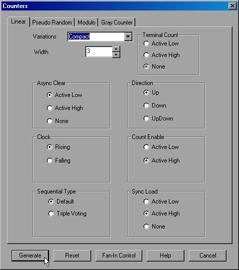
The parameters for the new counter can conveniently be set using the controls in the dialog window. The "Help" button provides more detailed information about the selected core and the meaning of its parameters. Since our counter should count from 0 to 7, a width of three bits must be specified under "Width".
Once all settings have been made, the "Generate" button starts the creation of the macro. Another dialog then appears in which the file name and type of the new core as well as the netlist format (VHDL, Verilog, EDIF) must be specified. For this example, "VHDL" is selected; a behavioral model is not required. The current project directory should always be kept as the destination so that the new macro appears in the ACTgen Core Builder workspace and can be edited there. After saving, the following files have been created (the dialog unfortunately does not close automatically and must be closed manually via "Cancel"):

my_cnt.vhd:
The VHDL description of the core. Contains the entity "my_cnt" (and the corresponding architecture) of the counter:

entity my_cnt is
 port( Data : in std_logic_vector(2 downto 0);
       Enable, Sload, Aclr, Clock : in std_logic;
       Q : out std_logic_vector(2 downto 0)) ;
end my_cnt;

my_cnt.gen:
This file stores the macro parameters, which can be modified with the ACTgen Core Builder.

my_cnt.log:
This log file contains all details of the selected parameters of the generated cores in plain text format.

Step 5:
The function of the created macro can be achieved using port mapping as usual in VHDL. For this purpose, a component of the counter entity must be created and instantiated, as demonstrated by the following code snippet:

Code snippet for integrating the core:

entity E_MY_DESIGN is
    port ( CLK:         in  std_logic;
           RST:         in  std_logic;
           STOP:        in  std_logic;
           LED:         out std_logic_vector(3 downto 0)
    );
end E_MY_DESIGN;

architecture A_BSP of E_MY_DESIGN is
type   t_zustand is (zLED1, zLED2, zLED3, zLED4);
...
component my_cnt is
    port( Data                        : in std_logic_vector(2 downto 0);
          Enable, Sload,  Aclr, Clock : in std_logic;
          Q                           : out std_logic_vector(2 downto   0)) ;
end component;
...
signal INT_ZUSTAND   : t_zustand;
signal tq : std_logic_vector(2 downto   0);
begin
...
 my_cnt_inst : my_cnt PORT MAP ( "000", '1', '0', '1', CLK, tq );
...
end A_BSP;

 

back to table of contents

---

Schematic Based Entry

Introduction

In addition to the text-based VHDL design level, Actel Libero gives the developer the option of creating a complete design in a graphical interface. Using a graphical editor (schematic editor), a circuit diagram can be designed that represents the structural description of a design at the logic level. Actel provides the adapted third-party tool "View Draw AE" from Mentor Graphics for this purpose. It can be launched directly from the Libero IDE and is therefore integrated into the design flow. In View Draw AE, the design is created with the mouse using menus, dialog boxes, toolbars and buttons. Since the two design levels (text-based and schematic-based) can also be combined (mixed-mode), the design flow can be accelerated and optimized.

How does work proceed in View Draw AE?

In the schematic editor "View Draw AE", the developer works with different blocks represented by graphic symbols arranged hierarchically on different levels. At the lowest level are the basic elements (primitives) such as logic gates AND, OR, etc. If several blocks are combined into one circuit diagram, a new block (composite block) is created, which can in turn be used in other designs. The functionality results from wiring and interconnecting the symbols used on one or more worksheets (sheets).

The interface of ViewDraw AE

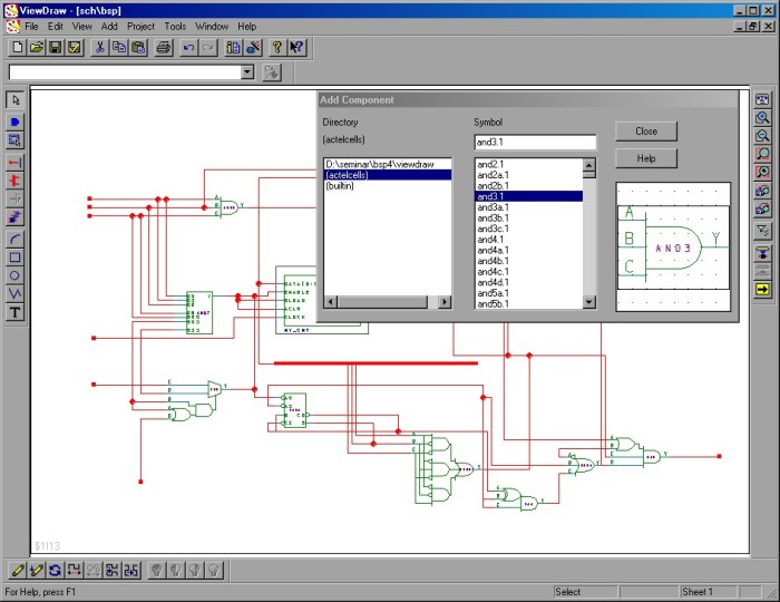
As shown in the screenshot, the View Draw AE window essentially consists of the white worksheet (in the center of the window) on which the schematic is assembled. Around the work area are various toolbar buttons that provide quick access to frequently used functions and drawing components. The upper toolbar offers important standard actions such as load, save, and copy & paste.

The left toolbar contains the most important elements for selecting new components or drawing wires, pins and buses. After clicking the "Add Component" button , the corresponding dialog window is displayed (as shown in the screenshot). There, a component can be selected from various directories and dragged onto the worksheet with the mouse. After clicking the "Net" button , the individual symbols can then be connected by drawing wires. The lower buttons contain drawing functions (for example for rectangles, circles, lines, etc.) to customize schematic symbols. The right toolbar contains various zoom functions. Relatively important is the bottom button in this toolbar, which allows switching between multiple worksheets. The lower toolbar contains functions for manipulating individual objects. This makes it possible to delete, rotate, scale, stretch or mirror blocks.

An example design - working with ViewDraw

The following example demonstrates how to create a schematic design with View Draw AE. The example design is intended to generate an output signal with the help of a 3-bit counter. The signal depends on the counter state and should only have a high level when one of the three bits is logically 1 or when all three bits are logically 1.
For this purpose, a simple logic evaluation of an ACTgen 3-bit counter with the following structure is created:

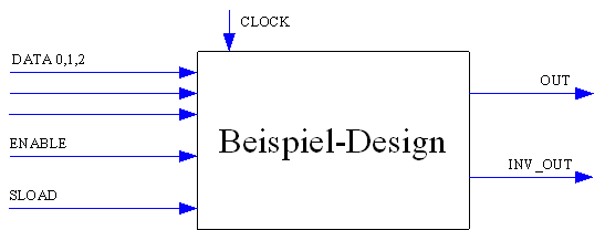
All input values refer to the internal 3-bit counter. If a binary value is applied to DATA 0,1,2, the counter can be initialized by applying a high level to the SLOAD input. In addition, the ENABLE signal must be set to "High" for the counter to operate.

At the output, only one logical signal "OUT" is routed externally; "INV_OUT" is the same signal, but inverted. "OUT" should always be high when exactly one of the three counter output bits is 1 or when all bits are set.

Step 1: Create a new schematic file

Once a new Libero project has been created, the "View Draw" button in the design flow can be clicked there, or alternatively the menu item "File->New" can be selected.

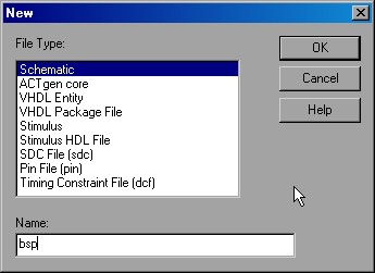
In the "New" dialog window that opens, the file type "Schematic" is selected and then a name (in the example "bsp") is entered for the new schematic object. After confirming with "OK", the program View Draw AE starts in a separate window and input can begin. Various settings (such as selecting a different color scheme in the "Color Palette" tab) can be made in advance via the menu item "Project->Settings".

Step 2: Add components

Now the placement and interconnection of the symbols can begin. Via the "Add Component" button on the left toolbar or by pressing the "c" key, the dialog window listing the individual components is opened:

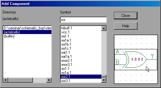
The left list (Directory) contains the available component libraries. The top directory (D:\seminar\schematic_bsp\...) refers to symbols of the current project. The entry "(actelcells)" contains the standard Actel components, from which an XOR symbol "xor2.1" (2 inputs, 1 output) with two inputs was selected for this example (as shown in the preview window). To use this symbol in the design, it must be dragged with the mouse from either the symbol name or the preview image onto the work area. The dialog window can remain open during the design process so it does not need to be reopened for each new symbol.

Since the counter in our example should have three output bits, a second XOR gate is required. This can either be dragged again from the "Add Component" dialog, or the symbol already placed on the worksheet can be copied:

Step 3: Copy components

To copy the first XOR gate, it is first selected with a left click. Then the CTRL key is held down while moving a copy of the selected object to the desired location on the worksheet. Alternatively, after selecting an object it can be copied with CTRL+C (or cut with CTRL+X) and then inserted again elsewhere with CTRL+V and a left mouse click.

For the inverted output "INV_OUT" in our example, besides the two XOR gates, an inverter is also needed for the inverting output. This component has the intuitive name "inv.1". (Instead of the two XOR gates, a 3-input XOR gate could of course also be used: "xor3.1").

Step 4: Connect components

After the symbols have been placed on the work area, they can now be connected. To do this, the "Net" button is first activated. The wires are then drawn with the mouse, starting each time at the symbol terminals:

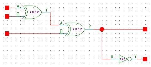
Tip: While drawing a wire, a support point can be inserted by clicking the right mouse button. This makes even complex routing possible.

Step 5: Define inputs and outputs (I/O)

For the inputs and outputs of a design (in and out of an entity) to be valid for description and simulation, they must be drawn in the schematic editor using the symbols "inbuf.1" and "outbuf.1". This is done according to the same principle as inserting the XOR components. The symbol is dragged onto the worksheet and connected to the corresponding signals.

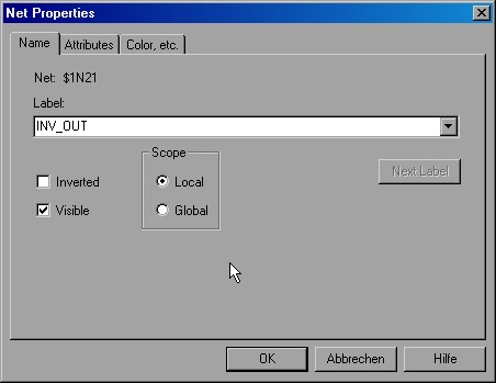
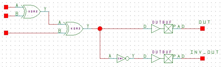
A short wire is then drawn in front of or behind the input/output buffer. Double-clicking this wire opens the "Net Properties" dialog, where a name can be entered for the input or output under "Label". In our design, these are initially only the outputs "OUT" and "INV_OUT" (the inputs will be added later together with the counter). The name is now displayed above the wire and can be moved with the mouse for better clarity:

Step 6: Add comments and graphic elements

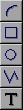To make the design clearer and more descriptive, it may be useful to add comments or graphic symbols (for example grouping boxes...) to the schematic. View Draw AE offers this possibility via the left toolbar. The drawing elements have no influence on the actual circuit.

Step 7: Generate and integrate a counter (ACTgen Core)

The counter is now to be integrated into the schematic circuit. First, as described in the previous chapter, a macro for the counter is generated using the ACTgen Core Builder (Counters->Linear->Compact->3-bit width) and added to the Libero project so that it appears in the Libero design hierarchy. There, the ACTgen module (here: my_cnt (my_cnt.vhd)) is right-clicked. In the context menu that appears, "Create Symbol" is selected - a new schematic symbol for the counter is generated and displayed in the File Manager under "Block Symbol files".

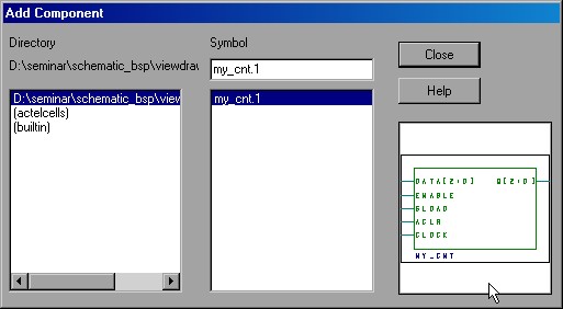
In the next step, the schematic is opened again in View Draw AE. As before, the "Add Component" button is used to display the "Add Component" dialog window. This time, however, the current project path is selected as the directory rather than "(actelcells)" (here: "D:\seminar\schematic_bsp\...").

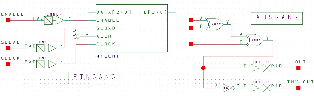
The counter appears as a symbol and can be dragged onto the worksheet. The simple inputs are then connected to the rest of the circuit (DATA and Q are wired later, because these are not single wires. These connections will later be combined via a bus).

Connecting a fixed low or high level (VCC, GND):
The ACLR input of the counter is not needed in our design and should always be logical 1 (1 because active low), since no clearing should occur. For this purpose it is connected to the symbol "vcc.1" (logical 0 would correspondingly be "gnd.1").

The expanded circuit with the corresponding inputs and wiring looks as follows:

Step 8: Manipulate objects

View Draw AE offers various ways to manipulate symbols in the schematic editor. A dedicated toolbar for this purpose is located at the bottom of the window. In particular, the rotate and mirror functions allow greater flexibility during schematic entry and clearer results.

Step 9: Create a bus

Finally, the two missing ports "DATA" and "Q" must be connected. Since this is a 3-bit counter, both ports are of the VHDL type "std_logic_vector(2 downto 0)" and should each be combined using a bus.

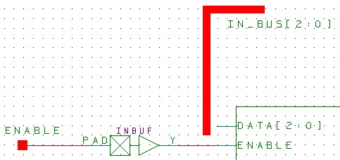
At first, the two buses are drawn freely into the circuit diagram without touching other signals. After activating the "BUS button" , drawing can begin. Once the bus has been drawn, it must be assigned a name by double-clicking it. This name must also indicate the bit width (-> std_logic_vector).

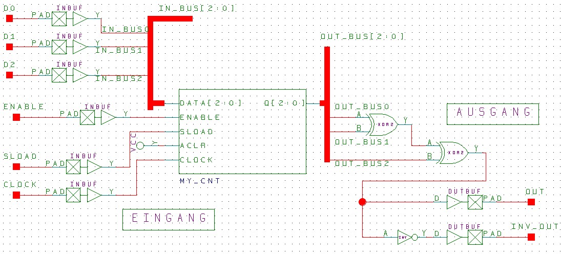
In our example, we choose the names "IN_BUS[2:0]" and "OUT_BUS[2:0]" and enter them in the "Label" field of the "Net Properties" dialog.

Next, the inputs and outputs are connected to the bus. This is done using the familiar net connection (via the "Net button"). Each connection must then be assigned a bus-specific name indicating which bit is meant. The name must match the bus name, but instead of the brackets the number for the desired bit is used (for example: "IN_BUS0", "IN_BUS1"...).

After adding the missing input signals and connecting the bus components, the example design under consideration has the following appearance:

Step 10: Save and test the circuit

Of course, the finished circuit must be saved (it is also safer to save several times during the process). This is done either via the save button, the menu item "File->Save", or the "Save+Check" function. The advantage of the latter is that the circuit is also checked additionally (for example whether all connections are correctly wired) and any errors found are reported.

Special functions in View Draw AE

Using multiple schematic worksheets (multi-page)

Since the space on a schematic worksheet is limited, View Draw AE allows the developer to combine multiple worksheets (sheets) into a multi-page design.

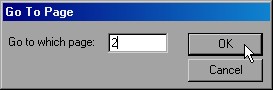
A new sheet can be created via the "Goto Page" button by switching to a new sheet that does not yet exist. A blank sheet is opened and a new schematic design can be started. The same button is used to switch back and forth between the individual worksheets.

What are Fubes?

With the help of Fubes, View Draw AE allows the developer to temporarily integrate a "black box" into the design. This is a block that is already fully wired into the design but does not yet provide any functionality. Fubes can be interpreted as "under construction" symbols. At a later stage in the design process, they are replaced by "real" modules, but during development they already occupy the correct position and can be assigned arbitrary connections or buses (the pins are updated automatically!). For clarity, the pins can also be given names.

Fubes can be placed on the worksheet using the "Fub" button .

 

Create and integrate new symbols

The schematic editor View Draw AE allows the developer to create their own symbols, which can then be used in later designs. In principle, four different types of symbols can be created - each for different application purposes:

1. Module Symbol (represents basic functions for the design)
2. Composite Symbol (contains a subordinate circuit / schematic)
3. Pin Symbol (represents a port or interface in a schematic design)
4. Comment Symbol (annotation symbol, graphic symbols for documentation purposes without circuit-specific properties)

These symbols are generated using the "Symbol Wizard" assistant, which can be launched via the corresponding button in the upper toolbar.

back to table of contents

---

Stimulus / Testbench - WaveFormer Lite

Introduction

Actel Libero includes the third-party tool WaveFormer Lite AE from SynaptiCAD. This program allows graphical input of individual signal waveforms, from which an HDL testbench can quickly and easily be exported. This testbench can be evaluated directly with the ModelSim simulator or adjusted manually beforehand (in VHDL code). Despite the restricted "Lite" version, in which not all functions are included, the tool is tailored to the Libero design flow. The signal information is read automatically from the HDL design and is already available when the program is launched.

Starting the program from Libero

WaveFormer Lite can be called directly within a Libero project in order to create a testbench. To do this, select the "Stimulus" button (shown on the left) in the design flow with a left mouse click. The tool then starts and automatically loads the signal information of the currently defined top-level design (which design unit that is can be set in the "Design Hierarchy" of Libero via right-click and the menu item "Set As Root"; if there is only one design unit, this option does not apply).

Defining startup options

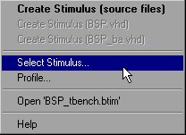
If the "Stimulus" button is right-clicked, a context menu appears with several options for stimulus generation. Via the entry "Select Stimulus", a dialog window can be opened in which the different existing stimulus files for the project can be activated. A new stimulus file can also be created or opened.

The graphical interface of WaveFormer Lite

WaveFormer Lite always opens in a separate window. The structure of the interface is demonstrated in the screenshot on the next page.
Below the menu bar, the program contains a button toolbar with the most important standard functions such as loading and saving as well as zoom options for displaying the signal waveforms (no. 1 in the screenshot).
In the client area, three different windows can be displayed and moved freely, so that either all three windows are visible at the same time or only one window is in the foreground:

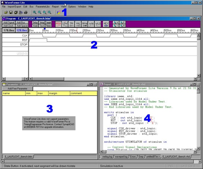
No. 2 - Diagram window:
This window is the heart of WaveFormer Lite. In the center, the signal waveforms are displayed or edited, while the associated signal names are shown on the left. Above them are buttons with important functions (for example for entering signal levels / transitions).

No. 3 - Parameter window:
This window can be ignored or minimized, since parameters are only enabled in the PRO version of WaveFormer.

No. 4 - Report window:
Various information and notes are displayed here. After exporting a testbench, the generated VHDL code can also be edited here. Since this can also be done in Libero, this window is of rather secondary importance.

Important options

Before beginning to create and edit the waveforms for individual design tests, some options should be adjusted, as the default settings cannot be used unchanged for every project.

Setting the base time unit

The base time determines the smallest time unit and influences all other time units in the entire program, since they are scaled as multiples of the base time. For this reason, it should be significantly smaller than the displayed time or the typical working time intervals. If a circuit operates in the nanosecond range (with regard to propagation delay / clock times), it is generally sensible to set the base time one unit smaller (that is, to picoseconds). On the one hand, accuracy is sufficient this way; on the other hand, good performance is ensured during internal processing.

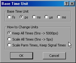
The base time can be set in a dialog (see figure above) opened via the menu item "Options->Base Time Unit". In the section "How to Change Units", you can also specify how already existing time values should be adapted to the new base time unit. If the timing diagram is still empty, this has no effect and can be ignored.

Display time unit

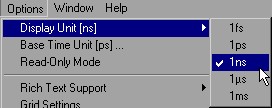
Via the menu item "Options->Display Unit", a time unit can be selected that predefines all visible time units in the working windows and in various input fields.

Working with WaveFormer Lite

Adding and removing signals

If WaveFormer Lite is started directly from the Libero design flow, all signal information from the current HDL description is already listed and can be selected with the mouse.
If a selected signal (or several selected signals) is to be removed, this can be done by pressing the "DEL" key. The signal disappears from the list and is not included in the testbench or remains uninitialized if it is an input signal. Signals can be added in the following ways:

1. By clicking the "Extract MUT ports" button , all signals can be loaded again from the design (the same state as after program startup). This function is very helpful if a signal has been removed accidentally.

2. Via the "Add Signal" button , a new signal can be added. It is automatically assigned a name (for example "SIG0") and added to the list. The new name consists of a fixed part (= prefix; e.g. "SIG") and an appended number. The used prefix (the default name) can be defined by right-clicking on the "Add Signal" button ; numbering is performed automatically:

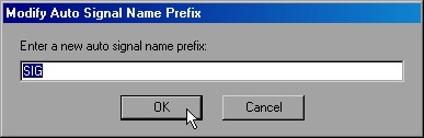
After the new signal has been added, its properties should be defined.

Defining signal properties

Double-clicking on a selected signal opens a new dialog window (see screenshot) in which the signal properties can be defined.

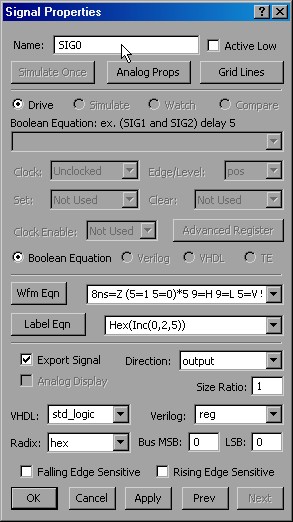
The most important options:

• In the upper field "Name", the signal name can be adjusted (duplicate names are not allowed in the testbench, even though WaveFormer Lite does not display an error message when creating them!)
• The checkbox "Export Signal" determines whether the signal will be included in the later testbench export (HDL code) or not.
• The selection menu "Direction" can be used to specify whether the signal should represent an input, output (or inout...).
• The selection field "Radix" can be used to choose the number base (for example binary, decimal, hex or ASCII) for display in the diagram.

An interesting feature is waveform generation via the "Wfm Eqn" button. First, an expression describing the signal waveform must be entered in the input field to the right. Clicking the button then converts the behavior described by the expression into a waveform and inserts it at the current position of the selected signal. The syntax consists of a list of time/value pairs separated by spaces (for example "8ns=1" to generate logical 1 for 8 nanoseconds).

Example of a clock behavior for 50ns with a period of 10ns:

5ns=0 5ns=1 5ns=0 5ns=1 5ns=0 5ns=1 5ns=0 5ns=1 5ns=0 5ns=1

Not only 0 and 1 are possible as values, but also: Z, V, H, L, X (std_logic).

In addition, it is valid to multiply a parenthesized expression. The clock behavior can therefore also be described more conveniently using one period repeated 5 times:

(5ns=0 5ns=1)*5

This shorter expression generates exactly the same waveform. Further information about the syntax can be found in the online help.

In a similar manner, signals in the diagram can be labeled by expression using the "Label Eqn" function. If the signal is a clock signal, these two functions are not available. Instead, the clock settings can be changed using the "Clock Properties" button.

Defining a clock signal

There are two ways to create a clock signal:

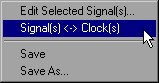
1. An existing signal can be converted into a clock signal. To do this, the desired signal must first be selected with a left click. Then, right-clicking on the signal name opens a context menu. Via the menu item "Signal(s) <-> Clock(s)", the signal is converted into a clock. The same method can be used in reverse to convert a clock back into a signal.

2. A new clock signal is added using the "Add Clock" button and is automatically assigned a name (for example "CLK0"), just like a "normal" signal. Here too, the name prefix can be changed by right-clicking. The next step is to adjust the clock settings.

Adjusting clock settings

The clock settings can be adjusted in the "Edit Clock Parameters" window (this window can be opened by double-clicking a clock signal name and then clicking the "Clock Properties" button). The most important options are:

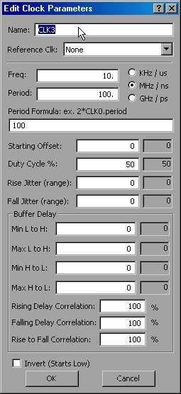
• In the upper input field "Name", the clock name can be changed
• In the Clock Rate section, the clock rate can be specified either as a frequency in the "Freq" field or as a period entered directly under "Period". Alternatively, the period can also be defined under "Period Formula" using an expression dependent on other quantities (one entry is sufficient; if rounding errors occur in connection with the clock frequency, the "Base Time Unit" must be adjusted.)
• In the Clock Properties section, an "Offset" can be specified that delays the waveform by the offset time. At time zero, a clock is normally "High" if no offset exists. (This behavior can be reversed with the "Invert (Starts Low)" button.)
• "Duty cycle" specifies the percentage of each period during which the clock signal remains "High". This influences the steepness of the edges. Another method for this is the "jitter" function, for both the positive and negative edges.

Copying and moving signals

For better clarity and structure, one or more signals within the WaveFormer Lite list can be moved by drag & drop with the mouse. To do this, the desired signal must be grabbed above or below the name and dragged up or down accordingly.

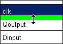
In addition, signals together with their waveform can be copied, cut and pasted again. As in Windows, this is done using the shortcuts CTRL+C, CTRL+X and CTRL+V, or alternatively via the "Edit" menu.

Drawing signal waveforms

This chapter describes drawing and manipulating waveforms. The required functions can be accessed via the toolbar buttons shown below:

Drawing a waveform (for example as shown below) in WaveFormer Lite is based on the principle that only the level changes need to be set in order to define the complete waveform unambiguously.

For this reason, the tool works with alternating function buttons. As can be seen in the upper screenshot, the "Low" button is active (red text). Above the "High" button there is also a small red "T", indicating that this is the state that will follow next. To create the waveform shown above, the first (positive) edge is defined by simply left-clicking in the signal row at the position of the first level change (approximately 6ns). The toolbar buttons switch automatically: the "High" button becomes active (red text) and the "Low" button gets the small red "T". It is then possible to continue directly to the right to the next (negative) edge (approximately 15ns). A left click sets the edge and the toolbar buttons toggle again. This can be repeated for the rest of the waveform.

To edit the waveform at the correct scale, the four right-hand zoom buttons can be used to zoom in and out.

Besides the classic levels, other states can also be drawn using the remaining buttons. Their meaning is as follows:

• HIGH, LOW
• TRIstate
• VALid, INValid
• WHI weak high, WLO weak low

It is also possible to choose the "toggle state" freely. To do this, the desired toggle state must first be clicked (it becomes red / active), then the partner state can be selected with a left click. When drawing level changes, the tool will now automatically alternate between these two states (if no alternation is desired, the desired state must be clicked twice). When creating signal waveforms with the mouse, the level changes inserted by clicking are automatically aligned to a grid. The grid spacing can be changed via the menu item "Options->Grid Settings->Signal Edge Grid".

The drawn waveform is automatically divided by the program into individual segments, each extending in width until the next level or state change. The following image shows a selected segment (green box):

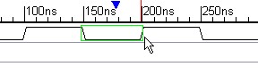
Each segment can be selected and edited. To do this, it must first be activated with a mouse click (green box), after which a new state can be selected via the toolbar buttons. The cursor can also be used to move the edges left or right.

A selected segment can be deleted with the "DEL" key.

A small segment can be created within a large segment by first selecting the large segment. Then click into the segment and move the cursor left or right while holding the mouse button down. Release the mouse button at the target position.

If a design works not only with the seven standard states but also with virtual states (such as integer, ASCII or enumeration types), these can be entered using the "Hex" button.

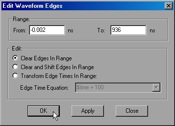
An important option, unfortunately somewhat "hidden", is found in the menu under "Edit->Edit Waveform Edges". Among other things, this makes it possible to modify all edges of a signal. Also very useful is the function "Edit->Right Click Delete Mode". It allows quick deletion of individual segments with a right click.

Adding a bus

WaveFormer Lite supports three types of buses: "Group Buses", "Virtual Buses" and "Simulated Buses".

1. Virtual bus:

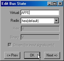
Virtual buses are represented by normal signals and can contain arbitrary information. The state of a virtual bus can either be defined via the "HEX" button or with the "VAL" button. For this, it is useful to click the "VAL" button twice so that it keeps its state (it is active, red, and marked with a small "T"). After drawing the individual segments, they must be selected. Then, after double-clicking a segment, the state can be entered in the "Edit Bus State" dialog. The lower screenshot shows the result:

Virtual buses are supported during testbench export and converted into corresponding VHDL code.

2. Group bus:

Several signals can be combined into a "group bus". The bus state is then directly coupled to the states of the subordinate signals. These no longer need to be set individually, but instead receive their state from the value of the bus. The following screenshot shows a "group bus" with the two associated signals "SIG0" and "SIG1":

The following steps combine several signals into a bus:

1. Select the individual signals (here "SIG0" and "SIG1") by clicking on the signal name. The order determines the corresponding bit in the bus. The signal selected first becomes the LSB, the last one becomes the MSB.
2. Once all signals are marked, press the "Add Bus" button and the "Choose Bus Type" dialog opens.
3. Select the radio button "Group Bus" and after confirming with "OK", the new bus appears in the diagram.

 

3. Simulated buses:

A simulated bus is only simulated and has no subordinate signals that may be changed. It is described by Boolean equations, but can only be used with the PRO version of WaveFormer.

Time button and delta button

The two buttons shown in the screenshot above the signal names display two different times (34.90ns / 25.00ns):

The left "Time" button with black text shows the current position of the mouse cursor in the timing diagram. The right "Delta" button with blue text shows the difference between the position of the mouse cursor and the blue "Delta Mark" (the small triangle above the time axis). Every time the left mouse button is released in the timing diagram, the "Delta Mark" is automatically placed at that position. This makes it very easy to measure distances between different points in a waveform.

Scrolling:
These two buttons can also be used to scroll quickly in long timing diagrams. If the left button is clicked, an absolute time value can be entered to jump to. If a time value is entered via the right button, the current view is scrolled relatively by the specified amount.

Import/Export - testbench generation

The most important function after creating all signal waveforms is exporting the timing diagram as a VHDL testbench, which is then used for simulation. This is done via the menu item "Import/Export -> Export Timing Diagrams As".

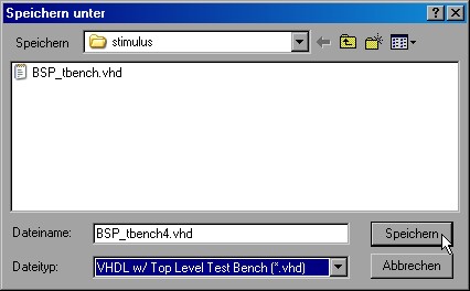
In the dialog shown, a name must be entered for the new testbench. For use in Actel Libero, the file type must absolutely be set to "VHDL w/ Top Level Test Bench (*.vhd)"!
After the new testbench has been generated, it is displayed in the WaveFormer Lite report window and can be reviewed or modified at the VHDL level. Then you can return to the Libero interface, where the new testbench also appears in the "Libero File Manager". Functional simulation can begin!

Outlook on the PRO version

The following table gives an overview of features and functions of the PRO version of WaveFormer that are not available or only available in limited form in the Lite version:

• An interactive simulator allows signal waveforms to be described using Boolean equations
• More options are available for describing propagation time, setup time, etc.
• All values in the timing diagram can be expressed using parameters.
• Macros allow flexible substitutions for signal names and values
• Additional versatile documentation functions are available that make waveforms clearer and easier to expand (for example marker & text functions)
• Various images / graphics can be generated in many formats
• Better import capabilities for waveforms from other manufacturers such as Altera Quartus
• Complete scripting functionality in the Perl language
• ...

Functional simulation

Starting ModelSim from Libero

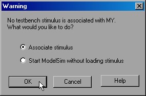
After the VHDL testbench has been exported from WaveFormer Lite and is available in Libero, the functional simulation can be performed. To do so, click the "Simulation" button (shown on the left) in the Libero design flow. In the dialog window "Warning" that follows, you are asked whether a testbench should be assigned to the simulator. We select "Associate stimulus" and confirm with "OK".

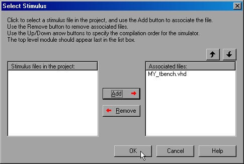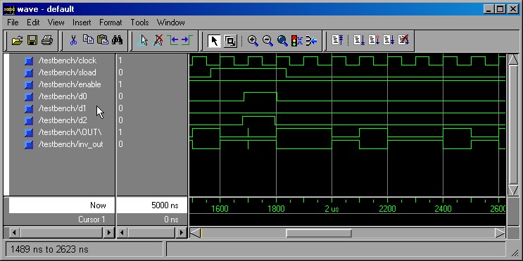
In the "Select Stimulus" dialog window, the testbench must now be selected and assigned using the "Add" button. After clicking "OK", the simulator "ModelSim" opens in a new window and visualizes the simulation result in a timing diagram, which should then be evaluated and checked.

The screenshot below demonstrates the simulation result for the schematic example design:

Simulation options

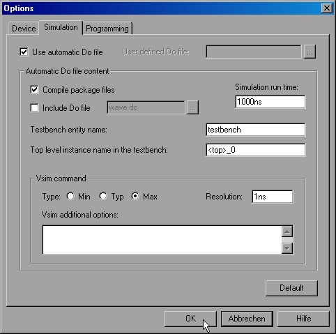
If the "Simulation" button in the Libero design flow is right-clicked, a new context menu appears. Via the menu item "Options", a dialog window opens in which important settings for the simulation process can be made. For example, the time span / simulation duration can be entered in the field "Simulation run time". The default value of 1000ns is often not sufficient. If the testbench has been modified, the name of the main entity may also have changed and can be corrected in the input field "Testbench entity name".

back to table of contents

---

Synthesis

Introduction

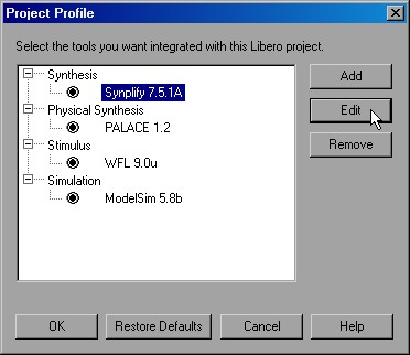
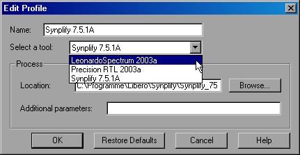
Once an HDL design has been created and its functionality has been successfully simulated with the help of a testbench, the design can be synthesized. The Actel Libero interface supports the following three synthesis tools from other manufacturers, adapted to the Libero design flow:

• Synplify from Synplicity
• LeonardoSpectrum from Mentor Graphics
• Precision RTL from Mentor Graphics

By right-clicking the "Synthesis" button in the Libero design flow and selecting the menu item "Profile", the desired synthesis tool can be selected in the dialog window that opens.

Since only Synplify AE from Synplicity is integrated into the standard Actel Libero design package, this chapter refers to that tool. Clicking the "Synthesis" button with the left mouse button opens the program from within Libero in a new window.

The interface of Synplify

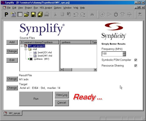
The figure below shows the interface of Synplify. Since the program was started from Libero, all project files are already selected and visible in a tree structure under "Source Files". The target platform (FPGA) has also already been transferred from Libero and can be found under "Target" again (in the example: "Actel eX").
The synthesis result is a netlist in EDIF format. Here too, the name is preset and can be found under the description "Result File".

The synthesis process

The actual synthesis process is started via the "Run" button. All status information as well as any warnings or errors that occur are recorded in a log file and can be displayed by clicking on it. In the middle of the window, the generated files (gate / RTL netlists, log files...) appear. Once synthesis has been completed, the result can be viewed and analyzed. However, since this is a restricted "Lite version", the possibilities are very limited and will not be discussed further here.

Via the toolbar buttons "RTL View" and "Technology View", an overview of the synthesis result can be displayed. A tree structure contains various elements such as used ports, nets, instances, each with fan-out. Unfortunately, the graphical assignment of the elements in the schematic cannot be opened in the restricted version.

back to table of contents

---

Notes on the tools

Fixing errors in an exported testbench

It can sometimes happen that the export testbench function of WaveFormer Lite generates VHDL code that causes the following error in the ModelSim simulator:

...
# ** Error: C:/bsp/stimulus/BSP_tbench.vhd(146): near "1.": Number must terminate with a digit.
...

This error occurs because WaveFormer Lite occasionally omits trailing zeros after the decimal point, as in the following line:

wait for 1.e-003 ns; 

If the line is corrected as follows, the simulation works again:

wait for 1.0e-003 ns;

Source of error: testbench export format

If ModelSim ever aborts in the log window with the following error message:

# ** Error: (vsim-3170) Could not find '../simulation/postsynth.testbench'.
# Error loading design
# Error: Error loading design

Then right-click the ModelSim icon in the Libero design flow, select "Options", and check the testbench entity name.

Source of error: ModelSim does not display output signals

If ModelSim does not display the output signals, the testbench was probably exported incorrectly: the format "VHDL (*.vhd)" was mistakenly selected during export instead of "VHDL w/ Top Level Testbench (*.vhd)"!

Source of error: ViewDraw does not start from within Libero

Depending on version, license and installation, ViewDraw AE may not start from within Libero. If you click the "ViewDraw" button in the design flow and enter a new schematic name, only an error message appears in the log window: "Unable to start ViewDraw AE...". This problem can be fixed as follows:

• Step 1: Save the current project and close Libero
• Step 2: Switch to the Libero installation directory and select the ViewDraw subfolder there (for example "C:\Program Files\Libero\ViewDraw")
• Step 3: In the ViewDraw folder there is a program called "configurator.exe", which can now be launched. The program resets the internal Windows path variables and then closes automatically.
• Step 4: Libero can now be started again. ViewDraw can then be launched from the design flow as intended.

back to table of contents

---

Help and further information

Useful documents on "Libero Design Creation/Verification"

• This documentation in Acrobat format (PDF)
• Mind map providing an overview of this documentation (PDF)
• PowerPoint presentation of the talk (PPS)

Links to the tool manufacturers

Manufacturer:	Tool:
Actel	Libero IDE
Mentor Graphics	ViewDraw AE (Schematic Based Entry) / ModelSim AE (Simulation)
Synplicity	Synplify AE (Synthesis)
SynaptiCAD	WaveFormer Lite AE (Stimulus)
Magma Design Automation	PALACE AE (Physical Synthesis)

Useful links related to VHDL

Page / Description:

Circuit synthesis with VHDL (FH Bielefeld)

VHDL related Usenet newsgroup

Application Specific Integrated Circuits

Kommentare 0